In this notebook we will demonstrate how chain together a set of process components using the Sequence class to create a new sequence model. We will then see how to run the model, plot some output, and dynamically change parameters mid-run.

Create the sequence model grid

The first step is to create a model grid (based on the landlab RasterModelGrid) on which we will run our new model.

import tqdm

from sequence import processes
from sequence.grid import SequenceModelGrid
from sequence.sequence import Sequence

The following code create a new grid with 100 vertical stacks that are each 1000 m in width. We then set the initial topoography (and bathymetry) for the model as well as setting sea level.

grid = SequenceModelGrid(100, spacing=1000.0)

grid.at_node["topographic__elevation"] = -0.001 * grid.x_of_node + 20.0

Create the process components

We now create the process components that will form the basis of the new model. All of the process components that come with sequence are located in the sequence.processes module.

Each of the processes components included with sequence are also landlab components but they don’t have to be. All that is necessary is that each component is an object that has a run_one_step method that accepts a single argument, dt, to indicate how long a time step it should be run for.

Components do not interact directly with one another but, instead, operate on landlab fields that are available to the other components through their common grid.

submarine_diffusion = processes.SubmarineDiffuser(
    grid,
    plain_slope=0.0008,
    wave_base=60.0,
    shoreface_height=15.0,
    alpha=0.0005,
    shelf_slope=0.001,
    sediment_load=3.0,
    load_sealevel=0.0,
    basin_width=500000.0,
)

fluvial = processes.Fluvial(
    grid,
    sand_frac=0.5,
    sediment_load=submarine_diffusion.sediment_load,
    plain_slope=submarine_diffusion.plain_slope,
    hemipelagic=0.0,
)

sea_level = processes.SinusoidalSeaLevel(grid, amplitude=10.0, wave_length=200000)

flexure = processes.SedimentFlexure(
    grid, method="flexure", rho_mantle=3300.0, isostasytime=0.0, eet=65000.0
)

compaction = processes.Compact(grid, porosity_min=0.01, porosity_max=0.5)

shoreline = processes.ShorelineFinder(grid, alpha=submarine_diffusion.alpha)

Create a new Sequence model

Create a new Sequence instance that will run sequenctially run the set of components. Sequence will run the processes in the order provided.

seq = Sequence(
    grid,
    time_step=100.0,
    components=[
        sea_level,
        compaction,
        submarine_diffusion,
        fluvial,
        flexure,
        shoreline,
    ],
)

Run the model for 3000 time steps.

for _ in tqdm.trange(3000):
    seq.update(dt=100.0)
seq.plot()

Dynamically change parameters

Increase sediment load

To demostrate how we can dynamically change parameters, we’ll now double the sediment input through the submarine_diffusion component.

submarine_diffusion.sediment_load *= 2

for _ in tqdm.trange(1500):
    seq.update(dt=100.0)
seq.plot()

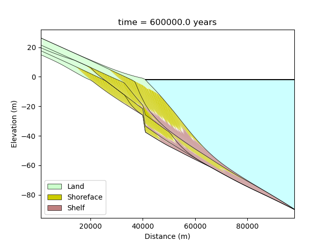
Create a vertical fault

As another example of dynamically changing parameters, we could create a fault at \(x=40 \rm km\),

grid.at_node["topographic__elevation"][grid.x_of_node > 40000] -= 10.0
grid.at_node["bedrock_surface__elevation"][grid.x_of_node > 40000] -= 10.0

seq.plot()

for _ in tqdm.trange(1500):
    seq.update(dt=100.0)
seq.plot()